A Pivot Table in Excel is a tool to analyze data. It is 5:30 PM on a Friday. Your manager comes to you with a USB drive and a look of desperation. He says, “I need a summary of all sales across our four regions broken down by product category and month. Also, can you show me which sales reps are hitting their targets? I need it for the 6:00 PM board meeting.

You open the file. It is a nightmare. Ten thousand rows of unformatted data are in front of you. Names, dates, amounts, and locations are all jumbled together in a soup.

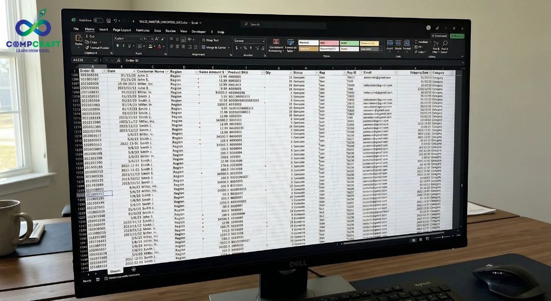
If you try to sort this or write individual formulas for every combination, you will be there until midnight. Your weekend plans are flashing before your eyes.

This is the moment where Advanced Excel skills stop being a nice thing to have on a resume and become a survival tool. Specifically, you need a Pivot Table in Excel. If you do not know how to use a Pivot Table in Excel, you are stuck in a labor loop. If you do know how to use a Pivot Table in Excel, that 6:00 PM meeting is not a threat. It is your time to shine.

The Secret Weapon of Data Analysts is the Pivot Table in Excel

So what actually is a Pivot Table in Excel? Think of it as a Smart Assistant that lives inside your spreadsheet. Imagine you have a box of mixed LEGO bricks. A Pivot Table in Excel is like a robot that can instantly sort those bricks by color, then by size, then by shape, and tell you how many of each you have. All without you having to touch a single brick yourself.

In terms of a Pivot Table in Excel is an interactive tool that lets you summarize large amounts of data without using a single formula. It. Rotates your data to look at it from different perspectives. You are not changing your data; you are just looking at it through a very powerful lens.

When people talk about an Excel course, the Pivot Table in Excel is often the moment when everything clicks. It is the bridge between being someone who knows Excel and someone who can actually drive business decisions.

Why the Pivot Table in Excel is Your Career Best Friend

A Pivot Table in Excel is because it saves you time.

Tasks that take an hour with formulas take seconds with a Pivot Table in Excel, especially when combined with strong fundamentals like those explained in VLOOKUP vs XLOOKUP: Which Excel Function Should You Use in 2026.

It is also very flexible. Want to see sales by City? Drag a box. Want to change it to sales by Year? Drag it back. It is effortless.

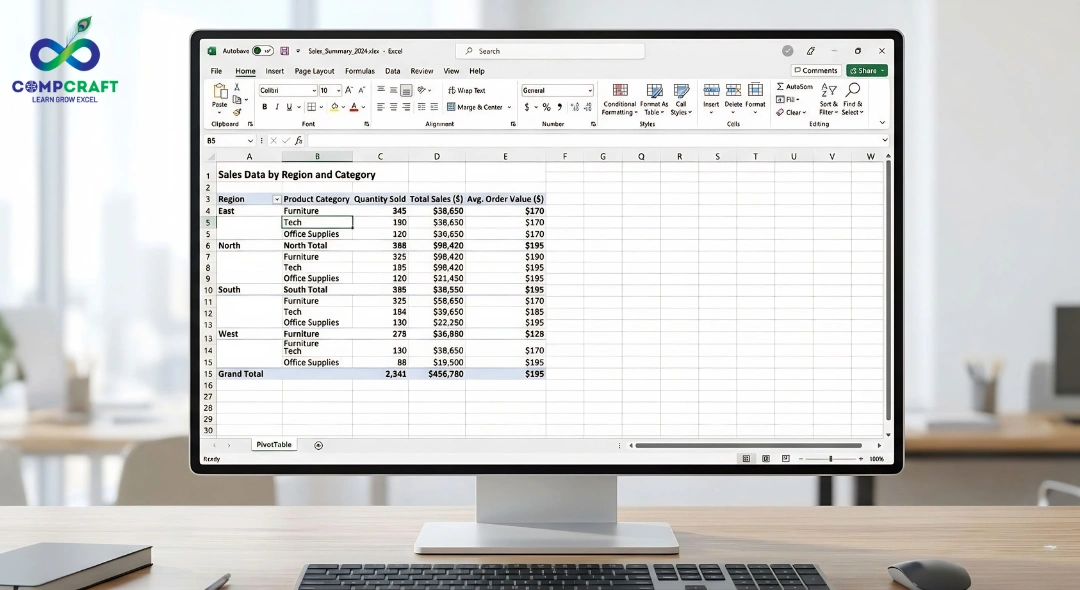
A Pivot Table in Excel is also very accurate. Since you are not typing formulas, you remove the risk of typing errors. It can take 50,000 rows. Turn them into a neat 5-row table that a CEO can actually understand.

Whether you are looking for an Excel course in Mumbai or you are already working in a high-pressure office, a Pivot Table in Excel will save you more time than any other feature in the software.

The Recipe for a Perfect Pivot Table in Excel

The Recipe for a Perfect Pivot Table in Excel is a four-step process.

1. The Prep Work

Your data needs to be in a tabular format. This means every column must have a header. No empty. Empty columns in the middle of your data. No merged cells. These are the enemies of Advanced Excel.

2. The Insertion

Click inside your data. Go to the Insert tab on the Ribbon. Click PivotTable. Excel will usually guess the range of your data correctly. Hit ‘OK’. You will be taken to a fresh blank worksheet.

3. The Four Quadrants

On the side, you will see the PivotTable Fields pane. This is your control center. You will see a list of your column headers and four empty boxes. Filters. Use this to clear out data you do not want to see. Columns. Whatever you drag here will show up as headers across the top. Rows. Whatever you drag here will show up as a list down the side. Values. This is for the numbers. Drag Sales. Quantity here.

4. The Pivot

This is the part. If you drag Region to Rows and Sales to Values, you see sales by region. If you then decide you want to see which products sold in those regions, just drag Product into the Rows box underneath Region. Suddenly, your table expands to show a breakdown.

Real Life Scenarios: From Chaos to Clarity

Let us look at how this plays out in a Mumbai office setting.

The HR Manager Scenario

Imagine you work in HR for a firm near Churchgate. You have a list of 500 employees, their departments, their joining dates, and their salaries. The boss wants to know the average salary per department to plan the budget.

The Pivot Fix

Drag Department to Rows and Salary to Values. Right-click the salary value, choose Value Field Settings, and change it from Sum to Average. Done in 15 seconds.

The Small Business Owner Scenario

You run a shop and track every sale in a spreadsheet. You want to know which day of the week is your busiest, so you can staff up.

The Pivot Fix

Drag Date to Rows and Transaction ID to Values. Set to Count. You will instantly see that Saturdays are 40% busier than Tuesdays.

Beginner Mistakes: And How to Avoid Them

Even if you have taken classes for Advanced Excel, it is easy to trip up. Here are the common pitfalls.

• Forgetting to Refresh. If you add data to your original list, the Pivot Table in Excel does not update automatically. You have to right-click the table and hit Refresh.
• Calculated Errors. Sometimes Excel defaults to Count of Sum. If your sales total looks weirdly small, check if it is just counting the number of rows or adding up the rupees.
• The Blank Row Mystery. If your Pivot Table in Excel shows a row called blank it means there are cells in your source data. Go back. Fill those in.

Pro Tips for the Workplace

Once you have mastered the basics of a Pivot Table in Excel, you can start using these moves.

• Slicers. These are buttons that let you filter your data with one click. They make your reports look like high-end dashboards.
• Pivot Charts. Turn your table into a bar graph or pie chart that updates instantly as you move your data around.
• Grouping Dates. You can right-click any date in your Pivot Table in Excel and Group it by Quarters or Years. This is a lifesaver for reporting.

Taking the Next Step

Mastering Pivot Tables in Excel is a step toward becoming indispensable at work, especially when combined with broader skills like those covered in How Excel Formulas Help in Getting Job-Ready Skills in Mumbai Companies.

It is about working not harder. While you can learn a lot by clicking, there is a certain logic to data that is best learned from experts who do this every day.

If you are looking for an Advanced Excel course in Charni Road, Mumbai, or perhaps you have been searching for Excel classes near Churchgate station, you are looking for more than a certificate. You are looking for the confidence to handle any data nightmare a boss throws at you.

At CompCraft, we focus on these job-ready skills. Whether you are looking for Advanced Excel classes near Charni Road Station or comprehensive Excel training in South Mumbai, our goal is to turn you into the person who finishes their work by 5:45 PM while others are still struggling with their sums.

Final Thoughts

Do not let data intimidate you. It is a bunch of numbers waiting for you to tell their story. If you are ready to level up your career, come find us at CompCraft. We will make sure you never fear a Friday afternoon deadline again.

Which Excel feature do you find most confusing? Let us talk in the comments. We might cover it in our guide.